How to remove column / rows grand total and sub-total from Excel 2013 pivot table

Pivot table is the fastest way to make flexible cross tab table and calculate sum, average, total, row / column grand total, sub-total, etc of data. It makes life much easier and most importantly the data is presented in organized structured piece of report. Apart from that the user can further filter the data to specific needs based on the requirements presentation.

However sometimes the Pivot table automatically calculate the rows and columns grand total as well as sub-total which is not needed as all the time. So here is the simple way how to remove the grand total and sub-total from the pivot table output.

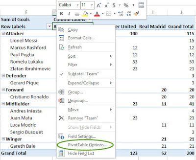
1. To remove grand total - mouse right click on the main header and click on "Pivot Table Options..."
2. Then click on the "Total & Filters" tab and uncheck the "Show grand total for rows" and "Show grand total for columns" then OK this will remove it from the pivot table output. To add it again simply repeat the same step and tick it back.







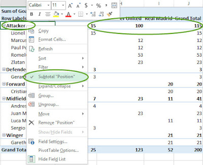
2. To remove the sub-total - mouse right click on the sub-total field header and left click to unchecked the Subtotal "Position"





How to remove grand total and sub-total from spreadsheet 2013 pivot table | ms.Excel 2013 | Microsoft Excel